The Dual Graph of a Mirror Design: Incidence Matrices and Eulerian Paths

From the Mirror Indicator Matrix to the 4-regular step graph and back

Introduction

In the companion module Mirror Matrices we treated the Mirror Indicator Matrix as a convenient design tool: its entries tell us where to place double-sided mirrors, and a 45° light ray bouncing off those mirrors produces a kolam or lusona.

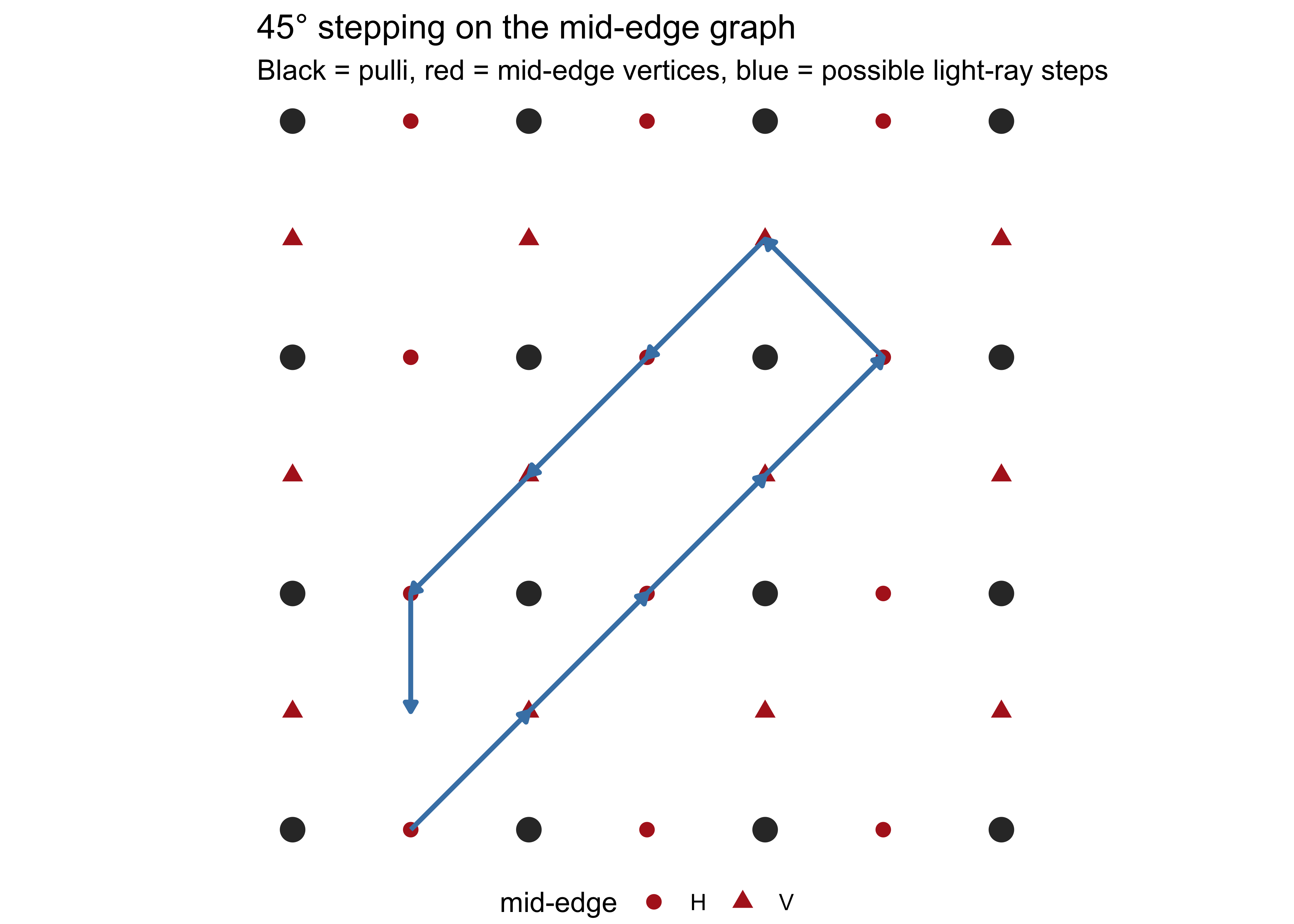
That construction has a precise graph-theoretic counterpart. The mid-points of the edges of the rectangular grid, together with the possible 45° steps that connect them, form a 4-regular graph (every vertex has degree 4). Placing a mirror is equivalent to choosing, at certain vertices, which pair of edges will be joined. The light-ray path is then an Eulerian path (or circuit) in a modified version of this graph.

Brick #1: Demonstrate 45° stepping on the mid-edge graph (the graph-theoretic counterpart of the mirror-curve construction)

library(ggplot2)

# ---- parameters ----
rows <- 4 # number of pulli rows
cols <- 4 # number of pulli columns
# pulli live at integer coordinates (0 .. cols-1, 0 .. rows-1)

# ---- 1. Pulli (dots) ----
pulli <- expand.grid(x = 0:(cols - 1), y = 0:(rows - 1))

# ---- 2. Mid-edge vertices of the step graph ----
# Horizontal mid-edges (between left-right neighbours)
h_mids <- expand.grid(x = 0.5:(cols - 1.5), y = 0:(rows - 1))
h_mids$type <- "H"

# Vertical mid-edges (between up-down neighbours)
v_mids <- expand.grid(x = 0:(cols - 1), y = 0.5:(rows - 1.5))
v_mids$type <- "V"

mids <- rbind(h_mids, v_mids)

# ---- 3. A few illustrative 45° steps ----
# Each step joins two mid-points that a light ray can travel between
# (here we hand-list a short chain that stays between the dots)
steps <- data.frame(
  x    = c(0.5, 1.0, 1.5, 2.0, 2.5, 2.0, 1.5, 1.0, 0.5),
  y    = c(0.0, 0.5, 1.0, 1.5, 2.0, 2.5, 2.0, 1.5, 1.0),
  xend = c(1.0, 1.5, 2.0, 2.5, 2.0, 1.5, 1.0, 0.5, 0.5),
  yend = c(0.5, 1.0, 1.5, 2.0, 2.5, 2.0, 1.5, 1.0, 0.5)
)

# ---- 4. Plot ----
ggplot() +
  # pulli
  geom_point(data = pulli, aes(x, y), size = 4, colour = "grey20") +
  # mid-edge vertices
  geom_point(data = mids, aes(x, y, shape = type), size = 2.5, colour = "firebrick") +
  # 45° steps (the edges of the step graph)
  geom_segment(
    data = steps,
    aes(x = x, y = y, xend = xend, yend = yend),
    arrow = arrow(length = unit(0.15, "cm"), type = "closed"),
    colour = "steelblue", linewidth = 0.9
  ) +
  coord_equal() +
  theme_void() +
  labs(
    title = "45° stepping on the mid-edge graph",
    subtitle = "Black = pulli, red = mid-edge vertices, blue = possible light-ray steps",
    shape = "mid-edge"
  ) +
  theme(legend.position = "bottom")

Figure 1: 45° stepping on the graph mid-edges

This module makes that correspondence explicit. We define the dual “step graph,” build its incidence matrix (displayed in LaTeX), show how the Mirror Indicator Matrix modifies the incidence structure, and recover the same curves we drew earlier—now as walks on a graph whose algebraic properties we can inspect directly. R code constructs the matrices; a p5.js sketch visualises the resulting Eulerian path.

The rectangular grid and its step graph

Let the pulli (dots) sit at the integer points ({0,1,,c-1} {0,1,,r-1}).

The step graph (G) is constructed as follows:

• Vertices of (G) are the mid-points of the unit-grid edges.
• Two vertices of (G) are joined by an edge when a 45° light ray can travel from one mid-point to the next without crossing a pulli.

In the absence of internal mirrors the graph is 4-regular. A monolinear mirror curve corresponds to an Eulerian circuit after the mirrors have been interpreted as forced pairings of edges.

Schematic of a 3×3 pulli grid with mid-edge vertices of the step graph marked

Incidence matrix of the step graph

The (oriented) incidence matrix (B) of a directed graph has one row per vertex, one column per edge, and [ B_{v,e} = \[\begin{cases} -1 & \text{if edge \(e\) leaves \(v\)},\\ +1 & \text{if edge \(e\) enters \(v\)},\\ 0 & \text{otherwise}. \end{cases}\]

]

For a tiny fragment of the step graph on a 3×3 pulli grid we may display the unoriented incidence matrix explicitly. Label four mid-edge vertices (v_1,v_2,v_3,v_4) and four possible 45° steps (e_1,e_2,e_3,e_4). Then

\[ B = \begin{bmatrix} 1 & 0 & 0 & 0 \\ 1 & 1 & 0 & 0 \\ 0 & 1 & 1 & 0 \\ 0 & 0 & 1 & 1 \end{bmatrix}. \]

(The precise numerical entries depend on the chosen orientation and labelling; the pattern of two 1s per column is universal for an ordinary graph.)

Building the matrix in R

# Toy incidence matrix matching the LaTeX display above
B <- matrix(c(
  1, 0, 0, 0,
  1, 1, 0, 0,
  0, 1, 1, 0,
  0, 0, 1, 1
), nrow = 4, byrow = TRUE)

rownames(B) <- paste0("v", 1:4)
colnames(B) <- paste0("e", 1:4)
print(B)

   e1 e2 e3 e4
v1  1  0  0  0
v2  1  1  0  0
v3  0  1  1  0
v4  0  0  1  1

# Vertex degrees (should be close to 4 in a fuller graph)
rowSums(B)

v1 v2 v3 v4 
 1  2  2  2 

The kernel of a signed version of (B) consists of the circulations—precisely the closed light-ray paths.

How the Mirror Indicator Matrix modifies the graph

Recall a typical Mirror Indicator Matrix from the companion module:

\[ M = \begin{bmatrix} 0 & 1 & 0 \\ 1 & 0 & 1 \\ 0 & 1 & 0 \end{bmatrix}. \]

Each non-zero entry imposes a linear constraint on the edge flows. For a vertical mirror that forces two opposite steps (e_i) and (e_j) to be paired we add the row

\[ \begin{bmatrix} \cdots & 1 & \cdots & -1 & \cdots \end{bmatrix} \]

to the incidence matrix, equating the two flow variables. The constrained matrix (B_M) therefore looks, in block form,

\[ B_M = \begin{bmatrix} B \\ \hline C_M \end{bmatrix}, \]

where the extra rows in (C_M) are read off directly from the 1s and 2s of (M).

# Example constraint row for one vertical mirror
C_M <- matrix(c(1, 0, -1, 0), nrow = 1)
B_M <- rbind(B, C_M)
rownames(B_M)[5] <- "mirror"
print(B_M)

       e1 e2 e3 e4
v1      1  0  0  0
v2      1  1  0  0
v3      0  1  1  0
v4      0  0  1  1
mirror  1  0 -1  0

# Dimension of the cycle space drops
qr(B)$rank

[1] 4

qr(B_M)$rank

[1] 4

Recovering the curve as an Eulerian path

Hierholzer’s algorithm (or any Eulerian-circuit routine) applied to the graph defined by (B_M) yields the sequence of mid-points visited by the light ray. Connecting those points with 45° segments reproduces the polygonal path of the earlier ray-tracer.

p5.js visualisation of the Eulerian path

The sketch below draws the pulli, a few mid-edge vertices, and an animated Eulerian circuit that respects a simple mirror constraint. Paste it into the p5.js Web Editor.

// Visualise step-graph vertices and an Eulerian path
// (simplified for a 3x3 pulli grid)

let cell = 80;
let margin = 100;
let path = [];
let t = 0;

function setup() {
  createCanvas(500, 500);
  // Hard-coded Eulerian circuit on mid-points (illustrative)
  path = [
    {x: 0.5, y: 0}, {x: 1, y: 0.5}, {x: 1.5, y: 1},
    {x: 1, y: 1.5}, {x: 0.5, y: 2}, {x: 0, y: 1.5},
    {x: 0.5, y: 1}, {x: 1, y: 0.5}, {x: 0.5, y: 0}
  ];
}

function draw() {
  background(252);
  translate(margin, margin);

  // Pulli
  fill(20); noStroke();
  for (let i = 0; i < 3; i++)
    for (let j = 0; j < 3; j++)
      circle(j * cell, i * cell, 12);

  // Mid-edge vertices of the step graph
  fill(180, 40, 40);
  for (let p of path) circle(p.x * cell, p.y * cell, 7);

  // Animated Eulerian path
  noFill(); stroke(30, 100, 190); strokeWeight(2.5);
  beginShape();
  let n = min(floor(t), path.length);
  for (let k = 0; k < n; k++)
    vertex(path[k].x * cell, path[k].y * cell);
  endShape();

  t += 0.15;
  if (t > path.length + 20) t = 0;
}

Animated Eulerian circuit on the step graph (screenshot placeholder)

Relation to classical network matrices

The signed incidence matrix of the step graph is a network matrix in the sense of Tutte and is therefore totally unimodular. Mirror constraints of the kind encoded by (M) preserve this property, which explains why integer light-ray circulations can be found by ordinary linear algebra.

Exercises

1. For a 2-by-2 grid of pulli write the full unoriented incidence matrix in LaTeX and verify every internal degree is 4.
2. Add one vertical mirror, append the corresponding constraint row, and compute the drop in rank.
3. Extract an Eulerian circuit from the constrained graph of the symmetric-cross example and plot it with the p5.js sketch above.
4. Project. Threshold a real-network adjacency matrix to obtain (M), build (B_M), and recover the kolam as an Eulerian circuit. Compare algebraic and geometric symmetries.

References

1. Paulus Gerdes. Lunda Geometry. Lulu, 2007.
2. Slavik Jablan et al. “Mirror-curves and knot mosaics.” arXiv:1106.3784.
3. William Tutte. “From matrices to graphs.” Can. J. Math., 1965.
4. Companion module Mirror Matrices: From Networks to Kolams, Lusona and Rangoli.

---

Editing the Mirror Indicator Matrix is exactly the same as editing the constraint rows of the incidence matrix of the step graph. Once that matrix is written down, every tool of linear algebra becomes a design operation.