How Contractive Maps Can Carry the Symmetries from Document 1
Iterated Function Systems (IFS)
An IFS is a finite set of contractive transformations (usually affine maps). Iterating them randomly produces a fractal attractor. When the set of maps is closed under a symmetry group, the attractor inherits that symmetry.
This connects directly to the fractal constructions you may have seen in the Fractals module (self-similar shapes built by repeatedly replacing a figure with smaller copies of itself).
Simple symmetric IFS in R
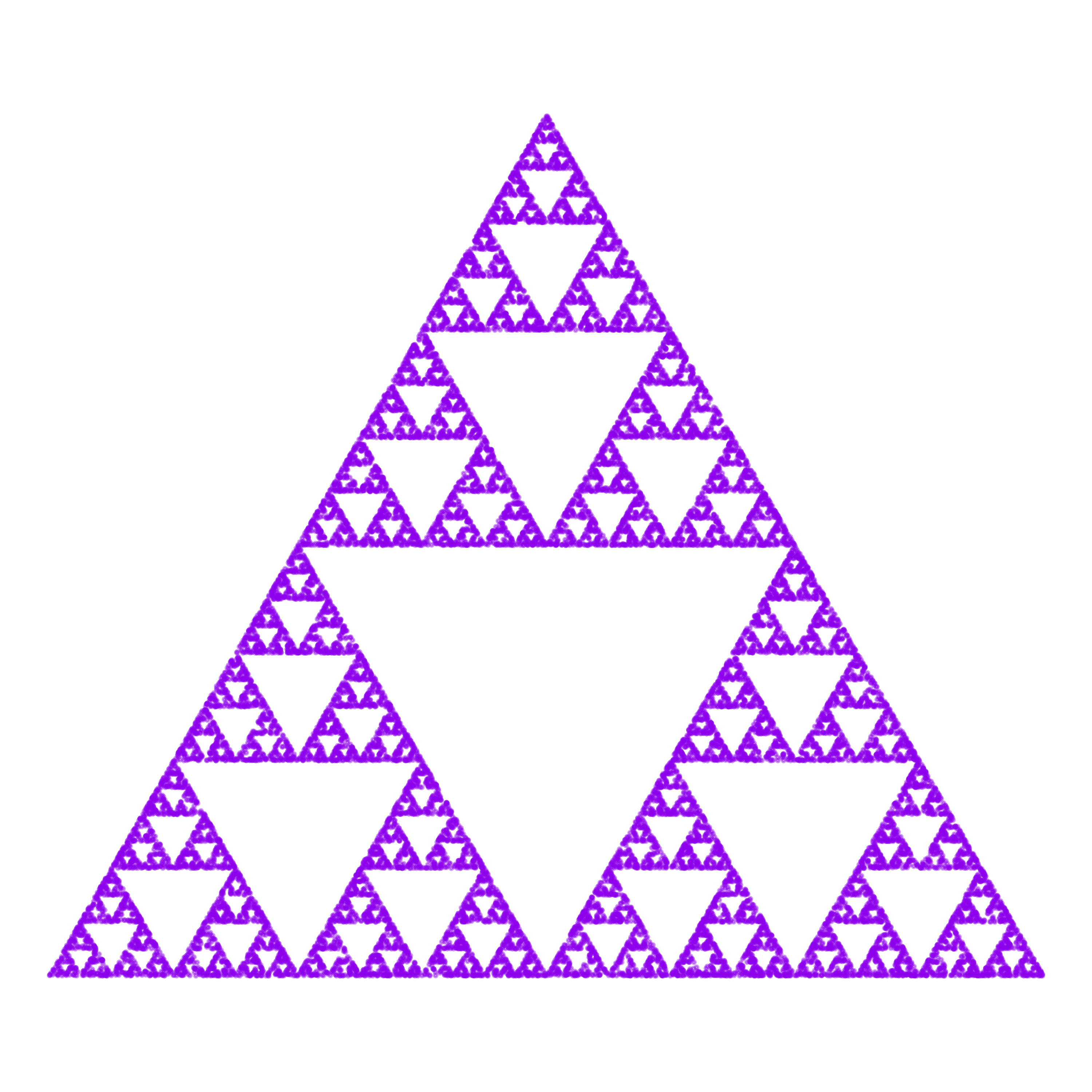
The following three maps generate a symmetric Sierpinski-like gasket with rotational symmetry of order 3.
# Three contractive maps (scale 0.5 toward the vertices)maps<-list(function(p)0.5*p+c(0, 0),function(p)0.5*p+c(0.5, 0),function(p)0.5*p+c(0.25, sqrt(3)/4))n<-25000pts<-matrix(0, n, 2)pts[1, ]<-c(0.3, 0.3)for(iin2:n){f<-sample(maps, 1)[[1]]pts[i, ]<-f(pts[i-1, ])}df<-as.data.frame(pts)names(df)<-c("x", "y")ggplot(df, aes(x, y))+geom_point(size =0.2, alpha =0.4, color ="purple")+coord_fixed()+theme_void()
IFS attractor with order-3 rotational symmetry
p5.js: live IFS with adjustable symmetry
A Simple Design Procedure
Choose the desired symmetry group
Decide on rotational order ( n ) or full dihedral ( D_n ). This is the same vocabulary as Document 1.
Select a fundamental domain
Pick a small set of “seed” points or a basic shape that will be copied by the group actions.
Define contractive maps that respect the group
For each group element ( g ), include a map of the form
[ f_g(p) = s g(p) + t ]
where ( s < 1 ) is a scale factor and ( t ) is a translation.
The collection ( {f_g} ) must be closed under the group action if you want the full symmetry.
Iterate randomly
Start from any point and repeatedly apply a randomly chosen map. After discarding the first few hundred iterates, plot the remaining points (or color by density).
Tune
Adjust scales, translations, and the probability of each map. Small changes produce large visual differences while the symmetry is preserved.
Example: adding reflections
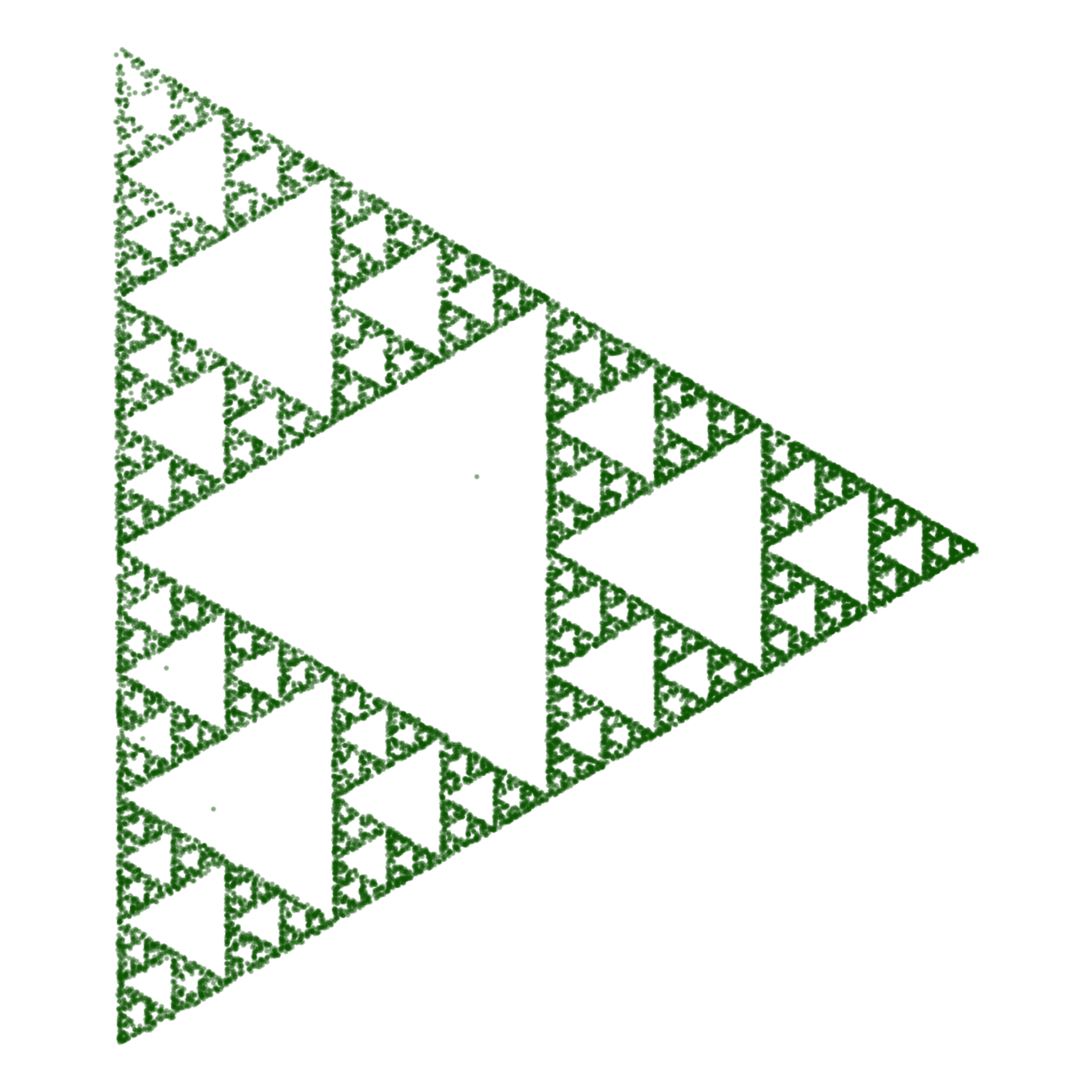
# Maps that include both rotations and a reflectionreflect<-function(p)c(p[1], -p[2])base_maps<-list(function(p)0.5*p+c(0.4, 0),function(p)0.5*p+c(-0.2, 0.35))n_iter<-20000pts<-matrix(0, n_iter, 2)pts[1, ]<-c(0.1, 0.1)for(iin2:n_iter){f<-sample(base_maps, 1)[[1]]p<-f(pts[i-1, ])if(runif(1)<0.5)p<-reflect(p)# randomly apply reflection# also rotate by 120° occasionally for order 3if(runif(1)<0.3){th<-2*pi/3R<-matrix(c(cos(th), -sin(th), sin(th), cos(th)), 2, 2)p<-as.numeric(R%*%p)}pts[i, ]<-p}df<-as.data.frame(pts)names(df)<-c("x", "y")ggplot(df, aes(x, y))+geom_point(size =0.15, alpha =0.35, color ="darkgreen")+coord_fixed()+theme_void()
Dihedral version (rotations + reflections)
Connection to Classic Fractals
Sierpinski triangle / carpet → special cases of the above procedure with particular scales and translations.
Koch curve, dragon curve, etc. can be rewritten as IFS and then symmetrized by adding the group actions.
The same design steps work whether you are building a deterministic L-system or a random IFS.
Once you have a set of maps that carry a symmetry, every iterate (and therefore the whole attractor) respects that symmetry. That is the bridge from Document 1 into generative fractal design.