Symmetry on Average

What Remains When the World Is Noisy

From Perfect Mirror to Average Mirror

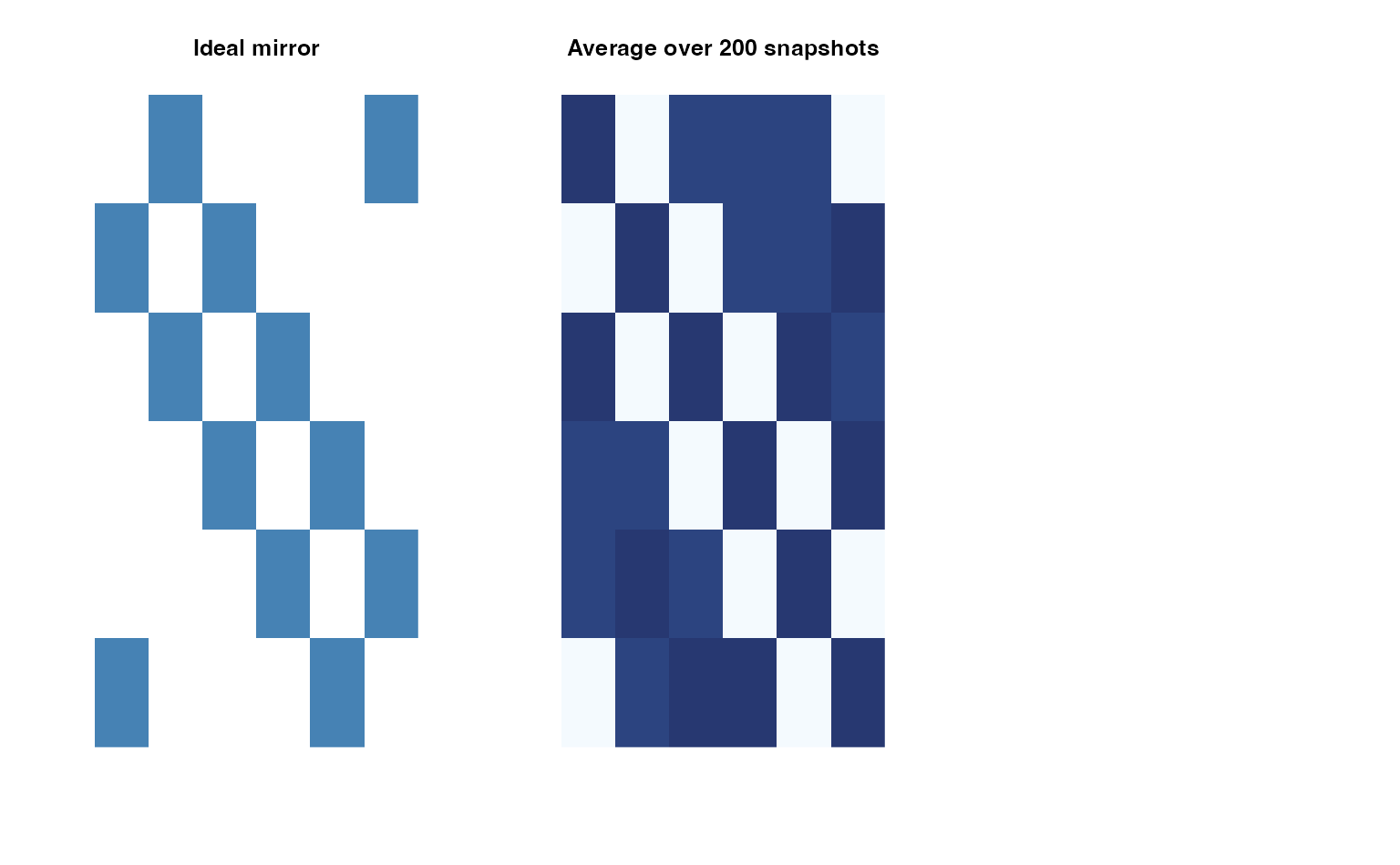
In the idealized world the matrix ( M ) satisfied ( M = M^) exactly.
In the real world edges are added and removed, directions flip, measurements are noisy. The instantaneous adjacency matrix is almost never symmetric.

Yet if we look at a long-run average — the density of visits, the time-averaged connection strength, the histogram of a chaotic orbit — a clear mirror symmetry can reappear. That is symmetry on average.

This is the idea from a classic paper Symmetric Chaos, by Frame and Golubitsky:

Download PDF File

Noisy adjacency that still averages to a mirror

# ideal mirror
ideal <- matrix(0, 6, 6)
ideal[1, 2] <- ideal[2, 1] <- 1
ideal[2, 3] <- ideal[3, 2] <- 1
ideal[3, 4] <- ideal[4, 3] <- 1
ideal[4, 5] <- ideal[5, 4] <- 1
ideal[5, 6] <- ideal[6, 5] <- 1
ideal[6, 1] <- ideal[1, 6] <- 1

# many noisy realizations
n_real <- 200
avg <- matrix(0, 6, 6)
for (k in 1:n_real) {
  noise <- matrix(rbinom(36, 1, 0.08), 6, 6)
  noisy <- pmax(0, pmin(1, ideal + noise - matrix(rbinom(36, 1, 0.08), 6, 6)))
  avg <- avg + noisy
}
avg <- avg / n_real

par(mfrow = c(1, 3))
image(t(ideal[6:1, ]),
  axes = FALSE, col = c("white", "steelblue"),
  main = "Ideal mirror"
)
image(t(noisy[6:1, ]),
  axes = FALSE, col = c("white", "firebrick"),
  main = "One noisy snapshot"
)

Error in `h()`:
! error in evaluating the argument 'x' in selecting a method for function 't': incorrect number of dimensions

image(t(avg[6:1, ]),
  axes = FALSE, col = hcl.colors(20, "Blues"),
  main = "Average over 200 snapshots"
)

Instantaneous noisy matrix versus its long-run average

Field and Golubitsky’s Design Method

Field and Golubitsky generate symmetric images by iterating a map that is equivariant under a chosen symmetry group (usually a cyclic or dihedral group of order ( m )).

The basic family of maps (in the complex plane) takes the form

[ z (+ |z|^2 + (z^m) + i) z + ^{m-1}. ]

• The polynomial is constructed so that it commutes with rotation by ( 2/m ) (and, when ( = 0 ), with reflections). That is the mathematical embodiment of the symmetry: if ( z ) is on the attractor then so is every rotated (and reflected) copy.
• Iteration of the map is chaotic for many parameter values: a single trajectory wanders aperiodically and never settles into a periodic orbit that itself possesses the symmetry.
• The density of a long trajectory (how often the orbit visits each pixel) nevertheless inherits the full symmetry of the map. Colouring by visit count therefore produces a picture whose symmetry is visible only “on average.”

This is precisely the passage from an idealized mirror constraint to symmetry-on-average in the presence of chaotic “noise.”

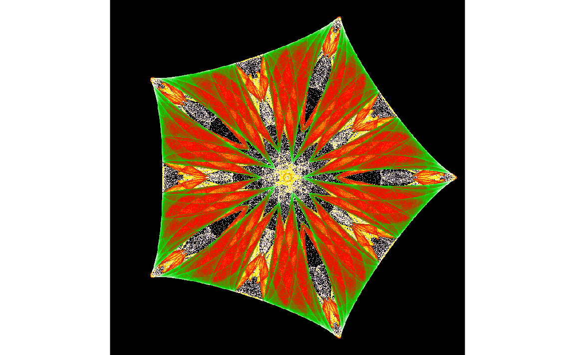
Emperor’s Cloak (pentagonal, ( m = 5 ))

A classic example uses the reduced form in which ( = -) (the complex logistic map plus a symmetry-breaking term):

[ z (- |z|^2) z + ^{4}. ]

library(grid)

# --- Parameters: Emperor's Cloak ---------------------------------------
n <- 5
lambda <- -1.806
alpha <- 1.806
beta <- 0
omega <- 0
gamma <- 1

cloak_step <- function(z) {
  (lambda + alpha * (Re(z)^2 + Im(z)^2) + beta * Re(z^n) + 1i * omega) * z +
    gamma * Conj(z)^(n - 1)
}

# --- Many orbits in parallel -------------------------------------------
set.seed(1)
n_orbits <- 20000
z <- complex(
  real = rnorm(n_orbits, sd = 0.1),
  imaginary = rnorm(n_orbits, sd = 0.1)
)
for (i in 1:500) z <- cloak_step(z) # burn-in

# --- Pass 1: bounds -----------------------------------------------------
L <- 0
zz <- z
for (i in 1:300) {
  zz <- cloak_step(zz)
  L <- max(L, abs(Re(zz)), abs(Im(zz)))
}
L <- L * 1.05

# --- Pass 2: 2D histogram ----------------------------------------------
N <- 800
counts <- numeric(N * N)
for (i in 1:1000) {
  z <- cloak_step(z)
  ix <- floor((Re(z) + L) / (2 * L) * N) + 1L
  iy <- floor((Im(z) + L) / (2 * L) * N) + 1L
  ok <- is.finite(ix) & is.finite(iy) & ix >= 1L & ix <= N & iy >= 1L & iy <= N
  counts <- counts + tabulate((iy[ok] - 1L) * N + ix[ok], nbins = N * N)
}

# --- Density -> colour --------------------------------------------------
d <- log1p(counts) / log1p(quantile(counts[counts > 0], 0.999))
d <- pmin(d, 1)
stops <- c(0, 0.10, 0.30, 0.50, 0.72, 1)
pal <- col2rgb(c("black", "#FFE9FF", "yellow", "red", "#00D600", "white"))
ch <- lapply(1:3, function(k) approx(stops, pal[k, ], xout = d)$y)
cols <- rgb(ch[[1]], ch[[2]], ch[[3]], maxColorValue = 255)

img <- t(matrix(cols, N, N))[N:1, ] # rows = y (top first), cols = x

# --- Draw on the active device (Quarto captures this) ------------------
grid.newpage()
grid.raster(img, interpolate = FALSE)

Figure 1: The Emperor’s Cloak symmetric icon (Field & Golubitsky).

library(symengine)
library(ggplot2)

# --- Parameters: Emperor's Cloak ---------------------------------------
n <- 5
lambda <- -1.806
alpha <- 1.806
beta <- 0
omega <- 0
gamma <- 1

# --- Symbolic map, using real/imaginary pairs --------------------------
x <- S("x")
y <- S("y")
cmul <- function(a, b) {
  list(
    re = a$re * b$re - a$im * b$im,
    im = a$re * b$im + a$im * b$re
  )
}
cpow <- function(a, k) {
  r <- list(re = S("1"), im = S("0"))
  for (i in seq_len(k)) r <- cmul(r, a)
  r
}

zn <- cpow(list(re = x, im = y), n) # z^n
zc1 <- cpow(list(re = x, im = -y), n - 1) # conj(z)^(n-1)

p <- lambda + alpha * (x^2 + y^2) + beta * zn$re
fx <- expand(p * x - omega * y + gamma * zc1$re)
fy <- expand(p * y + omega * x + gamma * zc1$im)

fx

(Add)   -1.806*x + 1.806*x*y^2.0 - 6.0*x^2*y^2 + 1.0*x^4 + 1.806*x^3.0 + 1.0*y^4

fy # inspect the expanded polynomials (optional)

(Add)   -1.806*y + 4.0*x*y^3 - 4.0*x^3*y + 1.806*x^2.0*y + 1.806*y^3.0

# --- Turn the symbolic polynomials into plain R functions ---------------
to_r_fun <- function(expr) {
  e <- parse(text = as.character(expr))[[1]] # "**" parses as "^" in R
  function(x, y) eval(e, list(x = x, y = y))
}
f_x <- to_r_fun(fx)
f_y <- to_r_fun(fy)

# Quick check against a direct complex-number calculation (optional)
z0 <- complex(real = 0.3, imaginary = -0.2)
z1 <- (lambda + alpha * Mod(z0)^2 + beta * Re(z0^n) + 1i * omega) * z0 +
  gamma * Conj(z0)^(n - 1)
all.equal(c(f_x(0.3, -0.2), f_y(0.3, -0.2)), c(Re(z1), Im(z1)))

[1] TRUE

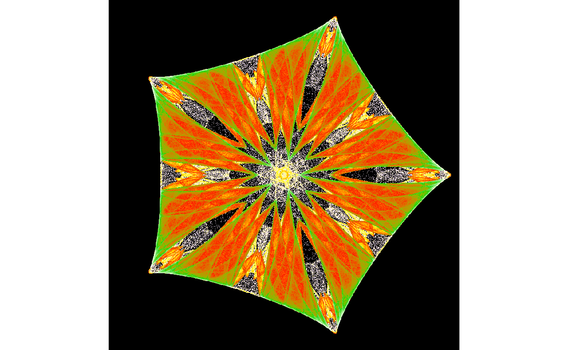
# --- Many orbits in parallel -------------------------------------------
set.seed(1)
n_orbits <- 20000
px <- rnorm(n_orbits, sd = 0.1)
py <- rnorm(n_orbits, sd = 0.1)

iterate <- function() {
  nx <- f_x(x = px, y = py)
  ny <- f_y(x = px, y = py)
  px <<- nx
  py <<- ny
}
for (i in 1:500) iterate() # burn-in

# Pass 1: bounds
L <- 0
sx <- px
sy <- py
for (i in 1:300) {
  nx <- f_x(x = sx, y = sy)
  ny <- f_y(x = sx, y = sy)
  sx <- nx
  sy <- ny
  L <- max(L, abs(sx), abs(sy))
}
L <- L * 1.05

# Pass 2: 2D histogram
N <- 800
counts <- numeric(N * N)
for (i in 1:1000) {
  iterate()
  ix <- floor((px + L) / (2 * L) * N) + 1L
  iy <- floor((py + L) / (2 * L) * N) + 1L
  ok <- is.finite(ix) & is.finite(iy) & ix >= 1L & ix <= N & iy >= 1L & iy <= N
  counts <- counts + tabulate((iy[ok] - 1L) * N + ix[ok], nbins = N * N)
}

# --- ggplot2 -------------------------------------------------------------
centres <- seq(-L, L, length.out = N + 1)[-1] - L / N
cloak <- data.frame(
  x = rep(centres, times = N), # ix varies fastest, matching the count index
  y = rep(centres, each = N),
  d = pmin(1, log1p(counts) / log1p(quantile(counts[counts > 0], 0.999)))
)

ggplot(cloak, aes(x, y, fill = d)) +
  geom_raster() +
  scale_fill_gradientn(
    colours = c("black", "#FFE9FF", "yellow", "red", "#00D600", "white"),
    values = c(0, 0.10, 0.30, 0.50, 0.72, 1),
    limits = c(0, 1), guide = "none"
  ) +
  coord_fixed(expand = FALSE) +
  theme_void() +
  theme(plot.background = element_rect(fill = "black", colour = NA))

Figure 2: The Emperor’s Cloak, built with symengine and drawn with ggplot2.

p5.js: live Emperor’s Cloak

Emperor’s Cloak accumulating in real time. The five-fold symmetry appears only in the density.

A second design (triangular symmetry)

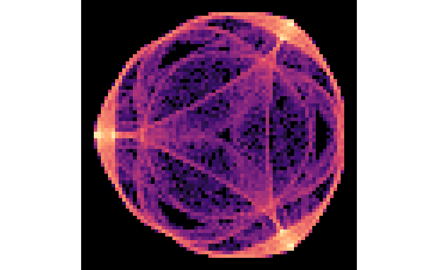
The same construction with ( m = 3 ) and different coefficients yields a triangular icon.

icon3 <- function(z, lambda = 1.5, alpha = -1.0, gamma = -0.8) {
  r2 <- Mod(z)^2
  (lambda + alpha * r2) * z + gamma * Conj(z)^2
}

n <- 100000
z <- 0.2 + 0.1i
pts <- complex(n)
for (i in 1:n) {
  z <- icon3(z)
  pts[i] <- z
}
pts <- pts[-(1:1000)]
pts <- pts[abs(pts) < 1.6]

df <- data.frame(x = Re(pts), y = Im(pts))

ggplot(df, aes(x, y)) +
  stat_bin2d(bins = 70) +
  scale_fill_viridis_c(option = "magma", trans = "log10", na.value = "black") +
  coord_fixed() +
  theme_void() +
  theme(
    legend.position = "none",
    plot.background = element_rect(fill = "black", color = NA)
  )

Triangular symmetric icon (m = 3)

The choice of the equivariant polynomial fixes the mathematical symmetry; the chaotic iteration supplies the randomness; the coloured density reveals the symmetry on average. That is the entire Field–Golubitsky design pipeline.

The Three-World Summary

World	Matrix relation	Visual character
Graphs & adjacency	( A ) arbitrary	Directed, possibly one-way
Idealized mirror	( M = M^) exactly	Perfect bilateral / dihedral
Real world	( [A] M )	Symmetry visible only on average

The artistic and design lesson is unchanged from the Field–Golubitsky pictures:
you may design with an equivariant rule (a “mirror” constraint) even when the underlying process is noisy or chaotic. The long-term image, the density, the average, will still carry the symmetry you imposed.

That is the practical bridge between the clean adjacency algebra and the hurly-burly of generative art.