library(ggplot2)

# 3×3 Mirror Indicator Matrix (only vertical mirrors)
# 1 = vertical, -1 = horizontal, 0 = empty
M <- matrix(c(
  0, 1, 0,
  1, 0, 1,
  0, 1, 0
), nrow = 3, byrow = TRUE)

rows <- nrow(M)
cols <- ncol(M)

# Pulli
pulli <- expand.grid(x = 0:(cols - 1), y = 0:(rows - 1))

# Midway vertical mirrors (where M == 1)
mirrors <- data.frame()
for (i in 1:rows) {
  for (j in 1:cols) {
    if (M[i, j] == 1 && j < cols) {
      mx <- j - 0.5
      my <- rows - i
      mirrors <- rbind(mirrors, data.frame(
        x = mx, y = my - 0.35, xend = mx, yend = my + 0.35
      ))
    }
  }
}

# 45° ray tracer that stays between the dots
trace_ray <- function(M, max_steps = 80) {
  rows <- nrow(M)
  cols <- ncol(M)
  x <- 0.5
  y <- 0
  dx <- 1
  dy <- 1
  path <- data.frame(x = x, y = y)
  for (s in 1:max_steps) {
    # outer walls
    if (x + dx * 0.5 < 0 || x + dx * 0.5 > cols - 1) dx <- -dx
    if (y + dy * 0.5 < 0 || y + dy * 0.5 > rows - 1) dy <- -dy
    # vertical-mirror test
    nx <- x + dx * 0.5
    if (abs(nx - round(nx)) < 1e-8) {
      cj <- round(nx) + 1
      ri <- round(y) + 1
      if (ri %in% 1:rows && cj %in% 1:cols && M[ri, cj] == 1) dx <- -dx
    }
    x <- x + dx * 0.5
    y <- y + dy * 0.5
    path <- rbind(path, data.frame(x = x, y = y))
    if (s > 8 && abs(x - path$x[1]) < 0.05 && abs(y - path$y[1]) < 0.05) break
  }
  path$y <- rows - 1 - path$y # flip for plotting
  path
}

path <- trace_ray(M)

ggplot() +
  geom_point(data = pulli, aes(x, y), size = 5, colour = "grey15") +
  geom_segment(
    data = mirrors, aes(x, y, xend = xend, yend = yend),
    colour = "firebrick", linewidth = 1.6
  ) +
  geom_path(data = path, aes(x, y), colour = "steelblue", linewidth = 1.2) +
  coord_equal() +
  theme_void() +
labs(title = "3×3 vertical-mirror matrix → closed curve embracing all 9 dots")Mirror Matrices: From Networks to Kolams, Lusona and Rangoli
A simple matrix that is simultaneously a graph, a mirror design, and a generative drawing
kolam
lusona
rangoli
graphs
matrices
symmetry
gerdes
Introduction
Across several cultures, people have developed beautiful ways of drawing continuous curves around grids of dots. In Tamil Nadu, women create kolams on the thresholds of their homes each morning, using rice flour to draw lines that loop around a set of dots called pulli in Tamil. In eastern Angola and neighbouring regions, the Tchokwe people draw sona (singular lusona) in the sand while telling stories; these drawings also embrace a rectangular array of dots, preferably with a single closed line. Similar ideas appear in various rangoli traditions across India.
What is striking is how often these drawings are monolinear (made of one continuous closed curve) and how frequently they display strong symmetry. Paulus Gerdes, working in the tradition of ethnomathematics, showed that a large and important class of these designs can be understood through a simple physical metaphor: imagine the outer boundary of the rectangle is mirrored, and that we place additional double-sided mirrors in the spaces between the dots. A ray of light that enters at 45 degrees will bounce around and eventually close on itself, tracing out exactly the kind of curve found in kolams and lusona. The same construction also produces the elegant black-and-white patterns Gerdes named Lunda designs.
In this module we introduce one ordinary matrix — we will call it the Mirror Indicator Matrix — that lets us hold all of these ideas at once. The entries of the matrix tell us where the mirrors go. Those same entries describe a network (a graph) on which the light ray is simply a walk. And because the matrix is just a table of numbers, the symmetries we already understand from linear algebra become design tools: if the numbers are symmetric in a certain way, the finished drawing will be symmetric in the corresponding geometric way. You can change a few entries and, almost without pause, obtain both a new network and a new kolam or lusona.
This module is designed to sit alongside the existing course page on Kolams and Lusona. The code below follows the same geometric convention shown in the figures there: the ray travels between the pulli at 45°, and the mirrors sit midway between adjacent dots.
The Mirror Indicator Matrix
Imagine we have decided on a rectangular grid of dots with ( r ) rows and ( c ) columns. Between these dots there are natural places where a short double-sided mirror can sit:
- A vertical mirror can be placed in the gap between two dots that are neighbours left and right.
- A horizontal mirror can be placed in the gap between two dots that are neighbours above and below.
- CHECK: Why not the other way around too?
For teaching purposes we gather all of this information into a single matrix ( M ) whose dimensions are roughly those of the grid itself. Each entry is a small whole number that records what (if anything) is present at that location:
| Entry | Meaning | What it does to a path | Quick symbol |
|---|---|---|---|
| 0 | nothing | the path may continue straight | · |
| 1 | vertical mirror | forces the path to bounce left or right | | |
| −1 | horizontal mirror | forces the path to bounce up or down | − |
| 2 | both (a crossing) | both kinds of reflection are present | + |
Here is a small concrete example for a 2-by-2 array of dots:
\[ M = \begin{bmatrix} O & - & O \\ 1 & & 1 \\ O & - & O \end{bmatrix} \]
According to the table above, every \(1\) means a vertical mirror and every \(−\) means a horizontal mirror. The matrix here contains both, so it places four mirrors: one H-mirror in the middle of the top row, one H-mirror in the middle of the bottom row, and two V-mirrors on each side of the middle row. The four mirrors form a kind of cross when you look at their positions. The light-ray path that results is still a single closed curve embracing all nine dots. Because the pattern of 1s looks the same after a 90° rotation of the matrix, the drawing inherits a corresponding rotational symmetry. The symmetry is already visible in the numbers; we do not have to impose it afterwards on the curve.
Why a single matrix is enough
The same table of numbers can be read in three complementary ways:
- As a network. The non-zero entries become the places where reflection is forced. Together with the outer walls they define a graph (technically a 4-regular graph on the mid-points of the grid edges). The light ray is simply a walk on this graph.
- As a kolam or lusona. When we smooth the polygonal path of the walk, we obtain precisely the kind of continuous curve traditionally drawn around the dots.
- As an algebraic object. Any symmetry we build into the numbers — making every row a palindrome, forcing the matrix to equal its own transpose, zeroing out a chessboard pattern, repeating a small block, and so on — is automatically inherited by the finished drawing. In this sense Gerdes’ geometric “mirror algebra” becomes ordinary matrix algebra that we can edit by hand.
When the matrix is entirely zero and the dimensions ( r ) and ( c ) are coprime (their greatest common divisor is 1), the construction recovers the classic single “plaited-mat” curve that winds around every dot. Adding mirrors in carefully chosen places — what Gerdes called “correct mirrors” — changes the visual character of the curve while leaving it monolinear.
From matrix to network to curve
The translation from one representation to the next is deliberately mechanical, so that you can move back and forth without losing the thread:
- Write down (or edit) the Mirror Indicator Matrix.
- Draw the grid of dots. Wherever an entry is non-zero, place a short double-sided mirror in the corresponding gap midway between the dots.
- Choose a starting mid-point on the boundary and send a ray inward at 45 degrees. The ray travels in the channels between the pulli. Whenever it meets a mirror or an outer wall it reflects (angle of incidence equals angle of reflection).
- Continue until the ray closes. The resulting polygonal path, once smoothed, is the kolam or lusona.
Because the matrix, the graph, and the curve are three readings of exactly the same data, a change made in a spreadsheet, an R matrix, or a JavaScript array appears at once in both the network diagram and the drawing.
Symmetry as matrix algebra
One of the pleasant surprises of this framework is that geometric symmetry becomes visible, and controllable, directly from the pattern of entries. A few correspondences that you can verify by hand or with the code below are:
| What you do to the matrix | What appears in the drawing |
|---|---|
| Make every row a palindrome | Vertical mirror symmetry |
| Force ( M = M^) (when the matrix is square) | Symmetry across the main diagonal |
| Arrange the entries so they look the same after a 180° turn | 180° rotational symmetry of the curve |
| Zero every entry where the row-plus-column index is even (or odd) | The alternating black-and-white structure of a Lunda design |
| Repeat a small block, or take a Kronecker product of simple 0-1 matrices | Hierarchical or self-similar rangoli patterns |
“Correct mirrors,” in Gerdes’ language, are exactly those changes to the matrix that do not increase the number of separate closed components. They correspond to placements that separate the inward-travelling strands of the original plaited-mat path from the outward-travelling ones.
Worked examples
Example 1 – The empty matrix and the classic plaited mat
Begin with a 5-by-3 grid and set every entry of ( M ) to 0. Because ( (5,3) = 1 ), a single light ray that starts at a boundary mid-point will eventually pass through every unit square and close on itself, producing one continuous curve that embraces all fifteen dots. This is the simplest monolinear lusona or kolam; many traditional designs can be seen as decorated versions of it.
If instead we had chosen dimensions that share a common factor — say 4-by-2 — the empty matrix would have produced two separate components. The greatest common divisor of the dimensions tells you, in the mirror-free case, how many closed curves you will need.
Example 2 – Vertical mirrors in a cross pattern
Return to the 3-by-3 matrix shown earlier:
\[ M = \begin{bmatrix} 0 & 1 & 0 \\ 1 & 0 & 1 \\ 0 & 1 & 0 \end{bmatrix} \]
All four non-zero entries are 1s, so we place only vertical mirrors. Their positions form a cross. The resulting curve is still a single closed loop. Because the pattern of 1s is unchanged under a 90-degree rotation of the matrix, the drawing itself shows the corresponding rotational symmetry. You can see that symmetry in the numbers before you draw the curve.
Example 3 – Chessboard mirrors and a Lunda design
Consider a slightly larger grid and zero every entry for which the sum of the row index and column index is even. The non-zero entries then sit only on the “black” squares of a chessboard colouring (or only on the “white” squares, depending on how you start the count). When the light-ray curve is drawn and the unit squares it passes through are coloured alternately black and white, one obtains precisely the kind of high-contrast Lunda design that Gerdes extracted from the mirror-curve construction. The chessboard condition on the matrix is doing the design work.
Example 4 – Imposing vertical symmetry by hand
Take any small matrix and replace each row by a palindrome (the row reads the same forwards and backwards). For instance, starting from a 4-by-5 grid you might arrive at
\[ \begin{bmatrix} 1 & 0 & -1 & 0 & 1 \\ 0 & 1 & 0 & 1 & 0 \\ -1 & 0 & 1 & 0 & -1 \\ 0 & 1 & 0 & 1 & 0 \end{bmatrix} \]
Every row is a palindrome, so the finished kolam must have a vertical axis of mirror symmetry. This is a reliable, low-effort way to guarantee symmetry while you experiment with different densities of mirrors.
R code: proper 45° ray between the pulli
The code below places the dots on the integer lattice and the mirrors midway between neighbouring dots (at half-integer coordinates), exactly as in the figures on the Kolams and Lusona page. The light ray travels at 45° so that it always stays in the channels between the dots; when it meets a mirror it reflects by reversing the appropriate component of its direction.
library(ggplot2)

# Mirror Indicator Matrix
#  1 = vertical mirror,  -1 = horizontal mirror,  2 = both,  0 = empty
M <- matrix(
  c(
    0, 1, 0, 1, 0,
    1, 0, 1, 0, 1,
    0, 1, 0, 1, 0,
    1, 0, 1, 0, 1,
    0, 1, 0, 1, 0
  ),
  nrow = 5, byrow = TRUE
)

rows <- nrow(M)
cols <- ncol(M)

# Dots (pulli) at integer locations
dots <- expand.grid(x = 0:(cols - 1), y = 0:(rows - 1))

# Mirrors placed midway between dots
mirrors <- data.frame()
for (i in 1:rows) {
  for (j in 1:cols) {
    val <- M[i, j]
    # vertical mirror between this column and the next, centred on the row
    if ((val == 1 || val == 2) && j < cols) {
      mx <- j - 0.5
      my <- rows - i
      mirrors <- rbind(mirrors, data.frame(
        x = mx, y = my - 0.4, xend = mx, yend = my + 0.4, type = "V"
      ))
    }
    # horizontal mirror between this row and the next, centred on the column
    if ((val == -1 || val == 2) && i < rows) {
      mx <- j - 1
      my <- rows - i - 0.5
      mirrors <- rbind(mirrors, data.frame(
        x = mx - 0.4, y = my, xend = mx + 0.4, yend = my, type = "H"
      ))
    }
  }
}

# ---- 45-degree ray tracer that stays between the dots ----
trace_ray <- function(M, max_steps = 400) {
  rows <- nrow(M)
  cols <- ncol(M)
  x <- 0.5
  y <- 0.0
  dx <- 1
  dy <- 1
  path <- data.frame(x = x, y = y)

  for (s in 1:max_steps) {
    nx <- x + dx * 0.5
    ny <- y + dy * 0.5

    # outer walls
    if (nx < 0 || nx > cols - 1) dx <- -dx
    if (ny < 0 || ny > rows - 1) dy <- -dy
    nx <- x + dx * 0.5
    ny <- y + dy * 0.5

    # vertical mirror crossing
    if (abs(nx - round(nx)) < 1e-6 && dx != 0) {
      cj <- round(nx) + 1
      ri <- round(ny) + 1
      if (ri >= 1 && ri <= rows && cj >= 1 && cj <= cols) {
        if (M[ri, cj] == 1 || M[ri, cj] == 2) dx <- -dx
      }
    }
    # horizontal mirror crossing
    if (abs(ny - round(ny)) < 1e-6 && dy != 0) {
      ri <- round(ny) + 1
      cj <- round(nx) + 1
      if (ri >= 1 && ri <= rows && cj >= 1 && cj <= cols) {
        if (M[ri, cj] == -1 || M[ri, cj] == 2) dy <- -dy
      }
    }

    x <- x + dx * 0.5
    y <- y + dy * 0.5
    path <- rbind(path, data.frame(x = x, y = y))

    if (s > 10 && abs(x - path$x[1]) < 0.1 && abs(y - path$y[1]) < 0.1) break
  }
  path$y <- rows - 1 - path$y
  path
}

path_df <- trace_ray(M)

ggplot() +
  geom_point(data = dots, aes(x, y), size = 3.5, colour = "grey15") +
  geom_segment(
    data = mirrors, aes(x, y, xend = xend, yend = yend),
    colour = "firebrick", linewidth = 1.4
  ) +
  geom_path(data = path_df, aes(x, y), colour = "steelblue", linewidth = 1.1) +
  coord_equal() +
  theme_void() +
  labs(title = "45° ray travelling between the pulli, reflecting off midway mirrors")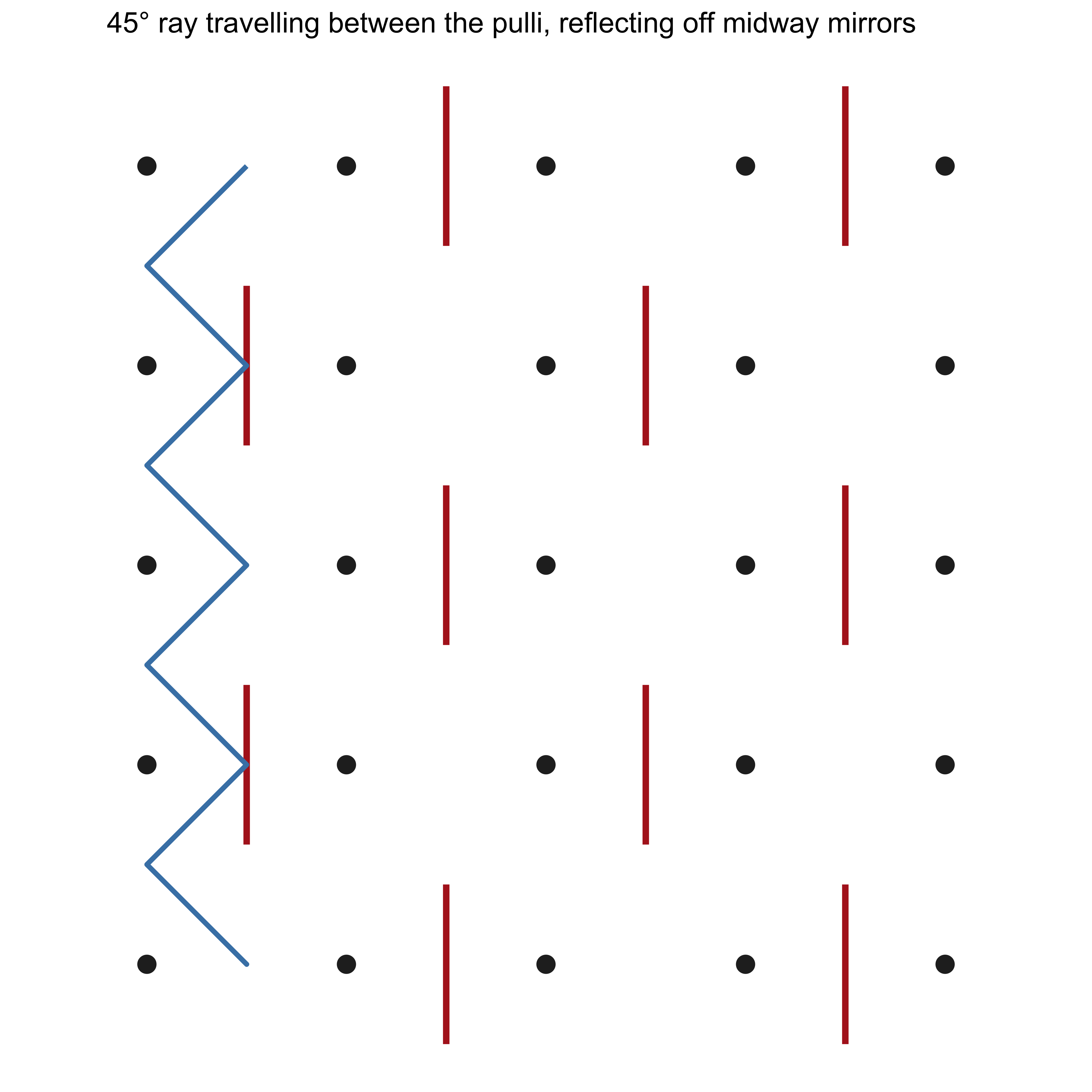
Edit the matrix M, re-run, and the blue path will thread between the black dots and bounce off the red mirrors exactly as in the Gerdes figures.
p5.js sketch: interactive 45° ray between the pulli
Paste into the p5.js Web Editor. The ray starts at 45° and stays in the channels between the dots; mirrors placed midway between adjacent pulli reverse the appropriate velocity component.
// 45° light ray between pulli, reflected by midway mirrors
// Matches the construction on the Kolams & Lusona page

let mirrorMatrix = [
  [0, 1, 0, 1, 0],
  [1, 0, 1, 0, 1],
  [0, 1, 0, 1, 0],
  [1, 0, 1, 0, 1],
  [0, 1, 0, 1, 0]
];

let rows, cols;
let cell = 70;
let margin = 90;
let path = [];
let t = 0;

function setup() {
  createCanvas(720, 720);
  rows = mirrorMatrix.length;
  cols = mirrorMatrix[0].length;
  generatePath();
}

function draw() {
  background(252);
  translate(margin, margin);

  // Pulli (dots) at integer lattice
  fill(20);
  noStroke();
  for (let i = 0; i < rows; i++) {
    for (let j = 0; j < cols; j++) {
      circle(j * cell, i * cell, 10);
    }
  }

  // Mirrors midway between adjacent dots
  stroke(190, 40, 40);
  strokeWeight(5);
  for (let i = 0; i < rows; i++) {
    for (let j = 0; j < cols; j++) {
      let v = mirrorMatrix[i][j];
      // vertical mirror between columns j and j+1
      if ((v === 1 || v === 2) && j < cols - 1) {
        let mx = (j + 0.5) * cell;
        let my = i * cell;
        line(mx, my - 22, mx, my + 22);
      }
      // horizontal mirror between rows i and i+1
      if ((v === -1 || v === 2) && i < rows - 1) {
        let mx = j * cell;
        let my = (i + 0.5) * cell;
        line(mx - 22, my, mx + 22, my);
      }
    }
  }

  // Animated 45° path
  noFill();
  stroke(30, 100, 190);
  strokeWeight(2.8);
  beginShape();
  let n = min(floor(t), path.length);
  for (let k = 0; k < n; k++) vertex(path[k].x, path[k].y);
  endShape();

  t += 0.6;
  if (t > path.length + 40) t = 0;
}

function generatePath() {
  path = [];
  // start between dots, direction 45°
  let x = 0.5 * cell;
  let y = 0;
  let dx = 1;
  let dy = 1;
  let steps = 0;
  const maxSteps = 600;

  while (steps < maxSteps) {
    path.push({ x, y });

    // next candidate position (half-cell step so we stay on diagonals)
    let nx = x + dx * cell * 0.5;
    let ny = y + dy * cell * 0.5;

    // outer boundary reflection
    if (nx < 0 || nx > (cols - 1) * cell) dx = -dx;
    if (ny < 0 || ny > (rows - 1) * cell) dy = -dy;
    nx = x + dx * cell * 0.5;
    ny = y + dy * cell * 0.5;

    // mirror tests (midway positions)
    let gj = nx / cell;          // continuous column
    let gi = ny / cell;          // continuous row

    // vertical mirror crossing
    if (Math.abs(gj - Math.round(gj)) < 0.05) {
      let cj = Math.round(gj);
      let ri = Math.round(gi);
      if (ri >= 0 && ri < rows && cj >= 0 && cj < cols) {
        if (mirrorMatrix[ri][cj] === 1 || mirrorMatrix[ri][cj] === 2) dx = -dx;
      }
    }
    // horizontal mirror crossing
    if (Math.abs(gi - Math.round(gi)) < 0.05) {
      let ri = Math.round(gi);
      let cj = Math.round(gj);
      if (ri >= 0 && ri < rows && cj >= 0 && cj < cols) {
        if (mirrorMatrix[ri][cj] === -1 || mirrorMatrix[ri][cj] === 2) dy = -dy;
      }
    }

    x += dx * cell * 0.5;
    y += dy * cell * 0.5;
    steps++;

    // rough closure test
    if (steps > 20 && dist(x, y, path[0].x, path[0].y) < cell * 0.3) break;
  }
}
Change any entry of mirrorMatrix and re-run: the red mirrors appear midway between the black pulli, and the blue ray threads between the dots, reflecting exactly as shown in the figures of the Kolams and Lusona module.
Using the two implementations together
- Use the R chunk when you want a static, publication-ready figure or to experiment with matrix algebra.
- Use the p5.js sketch when you want to watch the ray animate and to iterate quickly on mirror placements.
- In both cases the geometry now matches the construction on the existing Kolams and Lusona page: rays travel between the dots at 45° and bounce off mirrors placed midway between adjacent pulli.
Design techniques you can try immediately
- Start from the zero matrix on coprime dimensions and obtain the classic plaited-mat curve; then add mirrors one at a time and watch how the shape evolves while (if you choose “correct” places) the number of components stays equal to one.
- Guarantee vertical symmetry simply by editing each row until it is a palindrome; the drawing will follow.
- Build four-fold symmetry by writing a matrix that is unchanged under 90-degree rotation of its entries, then confirm the property in the sketch.
- Create a Lunda design by imposing a chessboard pattern of zeros and afterwards colouring the unit squares the curve visits.
- Take the adjacency matrix of a small real network (a group of friends, a set of campus buildings, a fragment of a transport map). Threshold it so that strong connections become 1s and weak ones become 0s. Interpret the result as a Mirror Indicator Matrix and turn the social or spatial graph into a kolam.
Exercises
- For a 4-by-4 grid, write a Mirror Indicator Matrix that has both horizontal and vertical mirror symmetry. First predict the appearance of the curve from the pattern of numbers, then check your prediction with either the R code or the p5.js sketch.
- Experimentally test the claim about “correct mirrors”: begin with an empty matrix on coprime dimensions (one component), then flip individual entries from 0 to 1 or −1 and count the number of closed curves that result. Which placements preserve monolinearity?
- Construct a chessboard-style matrix, generate the curve, and colour alternate unit squares to produce a Lunda design. Describe the symmetry you see.
- Project. Choose a real network with at least six nodes. Form its adjacency matrix, threshold it to a 0-1 Mirror Indicator Matrix, and produce both a conventional graph drawing and the corresponding kolam or lusona. Which symmetries of the original network survive in the drawing? Which new symmetries appear because of the way you thresholded?
References
- Paulus Gerdes. Lunda Geometry: Mirror Curves, Designs, Knots, Polyominoes, Patterns, Symmetries. Lulu, 2007. (See especially the chapters that introduce mirror curves and show how they generate Lunda designs.)
- Paulus Gerdes. Geometry from Africa: Mathematical and Educational Explorations. Mathematical Association of America, 1999.
- Paulus Gerdes. Sona Geometry from Angola: Mathematics of an African Tradition. Polimetrica, 2006.
- Gift Siromoney. Materials on kolam. https://www.cmi.ac.in/gift/Kolam.htm
- Venkatraman Gopalan and Brian Kevin VanLeeuwen. “A Topological Approach to Creating any Pulli Kolam.” arXiv:1503.02130, 2015.
- Papers by Gerdes in the electronic journal Visual Mathematics (Belgrade) on mirror curves, Lunda designs, and related matrices.
- The existing course module Kolams and Lusona.
Possible next steps: a companion module that develops the dual 4-regular graph and its incidence matrix more formally, or a small interactive widget in which the matrix is edited in an HTML table and both the R-style static plot and the p5.js animation update together.